Wisdom of the Crowd: Random Forest

We’ve learned about some algorithms in machine learning via which we can solve classification and regression problems. In the previous article, we learned how decision trees work, but the problem was that decision trees tend to overfit. But does there exist a use in which you can use decision trees to get even better results? Yes my friend there is an algorithm called Random Forest that uses not one but multiple decision trees to give a final prediction. Such a type of learning where you use multiple algorithms to get better predictive performance is called Ensemble Learning and we’ll learn about them.

Introduction to Random Forest

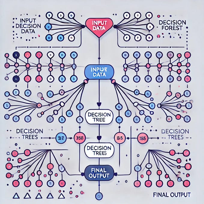
Random forests are an ensemble learning method for classification, regression, and other tasks that operates by constructing multiple decision trees at training time. For classification tasks, the output of the random forest is the class selected by most trees.

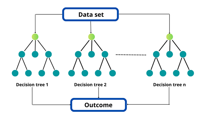
Intuition

Let’s take an example, It’s lockdown and all the classes have shifted to an online format and so have the exams. The teachers decided to create a difficult paper but allowed the students to help each other. Now our main character John tried to break into the group of intelligent students but they didn’t let him in. Poor John. But John is optimistic so he created his own group of average students which he called Examgers and devised a study plan to complete the syllabus for the exam.

Each and every student studied hard but on the day of the exam, the paper was quite a bit hard making it difficult to verify if one’s answer is the correct one. So they came up with a strategy, a brilliant one. They decided that everyone will attempt the same question and the answer that was in the majority will be the correct one. For example, If the question is fine if 256 is a perfect square then every member of Examgers will solve it and give their answers, and the answer given by the majority will be the final answer.

Let’s say 4 people said yes 256 is a perfect square and 2 said no it isn’t then the final answer would be Yes since it was decided by the majority. In the end, John’s group performed very well and the faces of intelligent students were a sight to see.

The way that John’s Group gave the exam is quite the same as that of the working of Bagging. Let’s understand bagging more in-depth.

Bagging

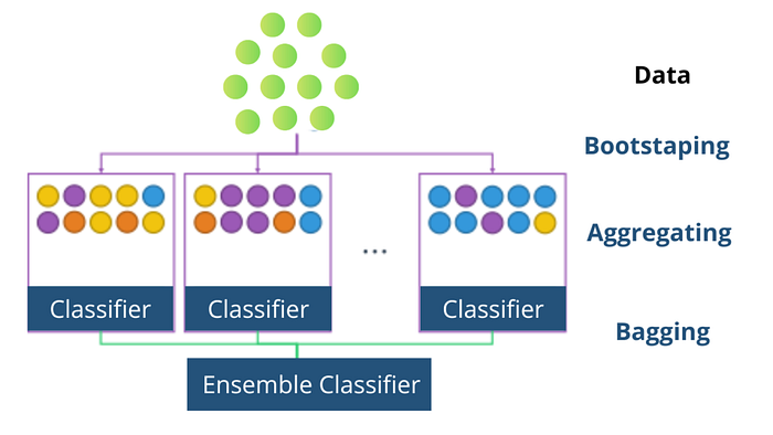
So in the previous articles, we saw how we can use various algorithms to predict a class and give its corresponding features of it. Bagging is an ensemble learning technique that combines the learning of multiple models to get a better-combined performance. It reduces overfitting and improves model stability. Bagging consists of 2 steps: Bootstrapping and Aggregation.

Bootstrapping

Bootstrapping is a technique by which we can create multiple smaller samples from a larger sample. One thing to note the smaller samples are created by drawing data points at random with repetition i.e. we might draw the same data point multiple times.

Let’s say we created N smaller samples, next thing we do is we’ll create N models and train them on the corresponding samples. For example, let’s say that we have N samples S1, S2, and S3 and we have created 3 models M1, M2, and M3. Then we’ll train M1 on S1, M2 on S2, and M3 on S3.

Now we have our trained models, but how do we combine their learning? After all, when given testing data each model may provide a different answer. That’s what aggregation is all about. Let’s take a look.

Aggregation

So let’s say we have testing data, t, and we predicted its class using our trained models. When predicting the class of testing data M1 predicted class 0, M2 predicted class 1, and M3 predicted class 0. Now we’ll take the max voted class i.e. class 0 as the final answer. This is the case for classification i.e. we take the max or majority voted class as the prediction of the ensemble model. In regression, we’ll take the average of all the predictions provided by the models and use that as the final prediction.

Working of Random Forest

Now Random Forest works the same way as Bagging but with one extra modification in Bootstrapping step. In Bootstrapping we take subsamples but the no. of the feature remains the same. But in Random forest, we also randomly select features to use in the smaller sub-sample. Let’s say we have data with 6 features(f1, f2, f3, f4, f5, f6) and 1000 data points. Then we create 3 smaller samples that look like this:-

• Sample 1: –
• Features: f1, f2, f3
• No. of rows: 500
• Sample 2:–
• Features: f1, f3, f6
• No. of rows: 500
• Sample 3:
• Features: f2, f4, f5
• No. of rows: 500

Now we’ll train 3 decision trees on these data and get the prediction results via aggregation. The difference between Bagging and Random Forest is that in the random forest the features are also selected at random in smaller samples.

Random Forest using sklearn

Random Forest is present in sklearn under the ensemble. Let’s do things differently this time. Instead of using a dataset, we’ll create our own using make_classification in sklearn. dataset. So let’s start by creating the data of 1000 data points, 10 features, and 3 target classes.

1

2

3

4

#loading the dataset

from sklearn.datasets import make_classification

X, Y = make_classification(n_samples = 1000, n_features = 10, n_classes = 3, n_clusters_per_class = 1)

In order to determine if our model performs well on data other than training data, we can split our data into two parts, one that we’ll use to train our model called training data, and one that we’ll use to test the performance of our model called testing data. train_test_split does exactly that we give it our data and test_size i.e. ratio of data to be used as test data.

1

2

3

4

5

#Importing train_test_split method

from sklearn.model_selection import train_test_split

#Splitting the data into train and test sets

x_train, x_test, y_train, y_test = train_test_split(X,Y, test_size = 0.3)

Now that we have our training and testing data let’s create our RandomForestClassifier object and train it on the training data. To train the data we use the fit() method like always. Let’s do it.

1

2

3

4

5

6

# Importing the RandomForestClassifier class

from sklearn.ensemble import RandomForestClassifier

#loading the data into the model

clf = RandomForestClassifier()

clf.fit(x_train, y_train)

Let’s make a confusion matrix for our predictions. You can find confusion_matrix in sklearn. metrics.

1

2

3

4

5

#Importing the confusion_matrix method

from sklearn.metrics import confusion_matrix

#Displaying the confusion matrix

print(confusion_matrix(y_test,clf.predict(x_test)))

Output:-
[[92  5  3]  
 [ 3 96  1]  
 [ 4  8 88]]

Advantages of Random Forest Algorithm

1. It reduces overfitting in decision trees and helps to improve the accuracy
2. Works well for both classification and regression problems
3. This algorithm is great for a baseline model.
4. Handles missing data automatically.
5. Normalizing of data is not required.

Disadvantages of Random Forest Algorithm

1. Computationally Expensive in random forest algorithm.
2. This algorithm takes time in fitting to build multiple decision trees.

Thanks for reading

Hope you enjoyed learning and got what you need.

Comment if you have any queries or if you found something wrong in this article.